
机器学习期末设计
预测锻炼期间燃烧卡路里的数据分析与建模
一、确定业务目标
本项目旨在通过分析锻炼相关数据,建立模型预测锻炼期间燃烧的卡路里量。这项研究具有重要的现实意义:
- 个性化健康管理:准确预测卡路里消耗可以帮助个人调整锻炼计划,达到健康减重或保持体重的目标。
- 健身效果评估:为健身爱好者提供量化的锻炼效果评估,优化锻炼方案。
- 智能健康设备开发:为智能手环、手表等健康监测设备提供更准确的卡路里消耗算法。
- 健康应用支持:为健康和健身应用提供更精准的能量消耗预测功能。
本项目的具体目标是:
- 分析各项身体指标和运动特征与卡路里消耗的关系
- 构建高精度的卡路里消耗预测模型
- 评估不同机器学习算法的预测效果
- 提供可用于实际应用的预测模型
二、获取数据
数据来源于Kaggle平台的"Calories Burnt Prediction"数据集。该数据集包含以下文件:
- train.csv:训练数据集,包含锻炼相关特征和卡路里消耗量
- test.csv:测试数据集,包含锻炼相关特征,需要预测卡路里消耗量
- sample_submission.csv:提交格式样例
数据集包含以下特征:
- id:记录ID
- Sex:性别(male/female)
- Age:年龄
- Height:身高(厘米)
- Weight:体重(千克)
- Duration:锻炼持续时间(分钟)
- Heart_Rate:心率(次/分钟)
- Body_Temp:体温(摄氏度)
- Calories:燃烧的卡路里(仅在训练集中提供)
这个是一个当前正在举办的比赛,地址:Predict Calorie Expenditure | Kaggle
三、数据预处理和探索性分析
3.1 数据预处理
数据预处理阶段包括以下步骤:
-
数据加载与检查:
- 加载训练和测试数据集
- 检查数据集大小和基本信息
- 查看数据类型和统计摘要
1
2
3
4
5
6
7
8
9
10
11
12
13
14
15
16
17
18
19
20
21
22
23
24
# 1. 数据获取
train_data, test_data = load_data()
# 2. 数据预处理
train_data = preprocess_data(train_data)
test_data = preprocess_data(test_data, is_train=False)
# 加载数据
def load_data():
"""
加载训练集和测试集数据
Returns:
tuple: (训练数据, 测试数据)
"""
try:
print("正在加载数据...")
train_data = pd.read_csv('train.csv')
test_data = pd.read_csv('test.csv')
print(f"训练集大小:{train_data.shape}, 测试集大小:{test_data.shape}")
return train_data, test_data
except Exception as e:
print(f"加载数据时出错:{e}")
raise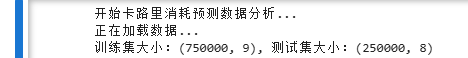
读取这个数据的前五行:
1
2
3
4
5
# 读取数据
train_data = pd.read_csv('train.csv')
# 显示前五行
print(train_data.head())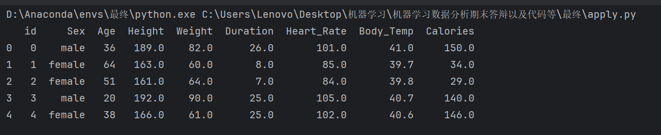
1
2
3
4
5
6
7
8
9
10
11
12print("正在进行数据预处理...")
# 创建数据副本,避免修改原始数据
df = data.copy()
# 显示数据基本信息
print("\n数据基本信息:")
print(df.info())
# 显示数据统计摘要
print("\n数据统计摘要:")
print(df.describe())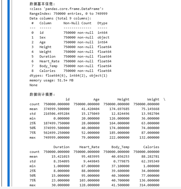
-
缺失值处理:
- 检查各特征的缺失值
- 使用适当的方法填充缺失值(若有)
1
2
3
4
5
6
7
8
9
10
11
12
13
14
15
16
17
18
# 检查缺失值
print("\n检查缺失值:")
missing_values = df.isnull().sum()
print(missing_values[missing_values > 0])
# 处理缺失值(如果有)
if df.isnull().sum().sum() > 0:
# 对数值型特征使用均值填充,分类特征使用众数填充
num_features = df.select_dtypes(include=['float64', 'int64']).columns
cat_features = df.select_dtypes(include=['object']).columns
for col in num_features:
if df[col].isnull().sum() > 0:
df[col].fillna(df[col].mean(), inplace=True)
for col in cat_features:
if df[col].isnull().sum() > 0:
df[col].fillna(df[col].mode()[0], inplace=True) -
特征编码:
- 将分类特征(如性别)编码为数值形式
- 男性编码为1,女性编码为0
1
2
3
4
5
6
7
8
9
10
11
# 性别编码:将性别特征转换为数值
if 'Sex' in df.columns:
df['Sex'] = df['Sex'].map({'male': 1, 'female': 0})
# 删除ID列,因为它不是预测的特征
if 'id' in df.columns:
df = df.drop('id', axis=1)
# 显示处理后的数据信息
print("\n预处理后的数据信息:")
print(df.info())
-
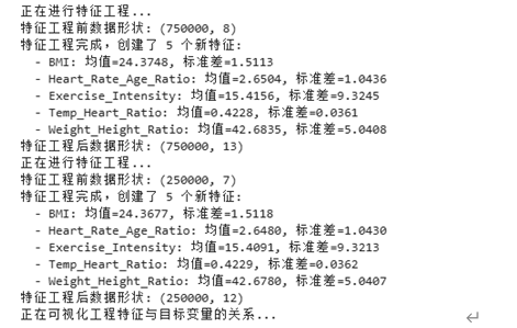
特征工程:
- 使用StandardScaler对数值特征进行标准化处理(模型训练和评估当中)
- 使模型训练更稳定,提高收敛速度
1 | # 特征工程 |
3.2 探索性数据分析
代码:
1 | # 探索性数据分析 |
探索性数据分析阶段包括以下内容:
-
目标变量分析:
- 卡路里消耗的分布情况
- 异常值检测
-
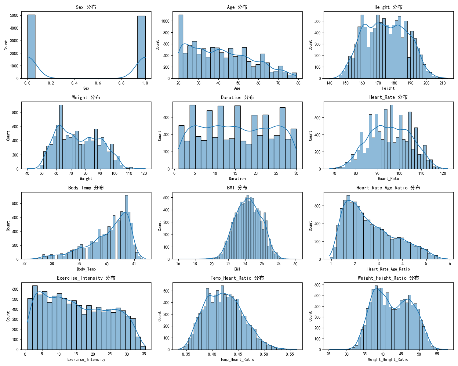
特征分析:
- 各特征的分布情况
- 箱线图检查异常值
-
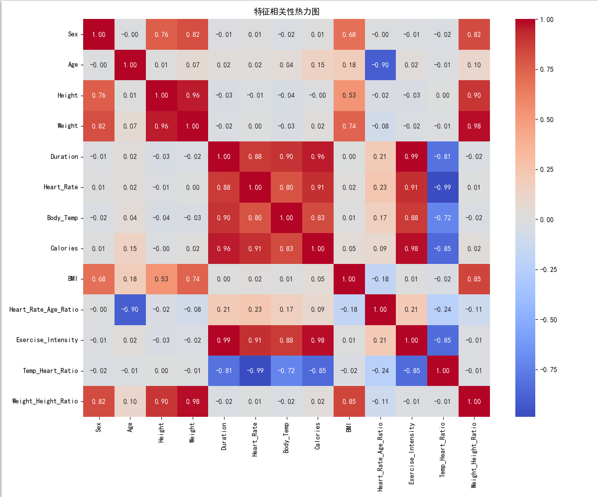
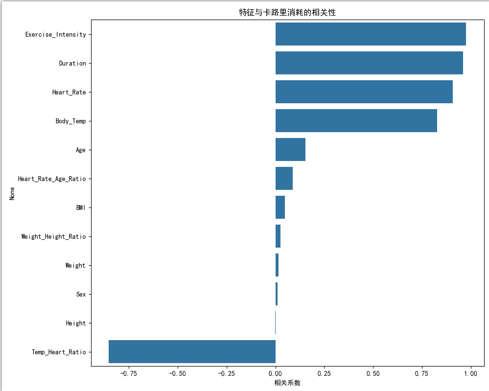
相关性分析:
- 特征间的相关性热力图
- 各特征与卡路里消耗的相关性
-
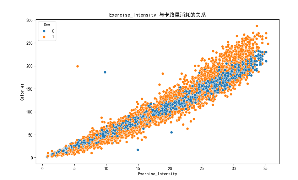
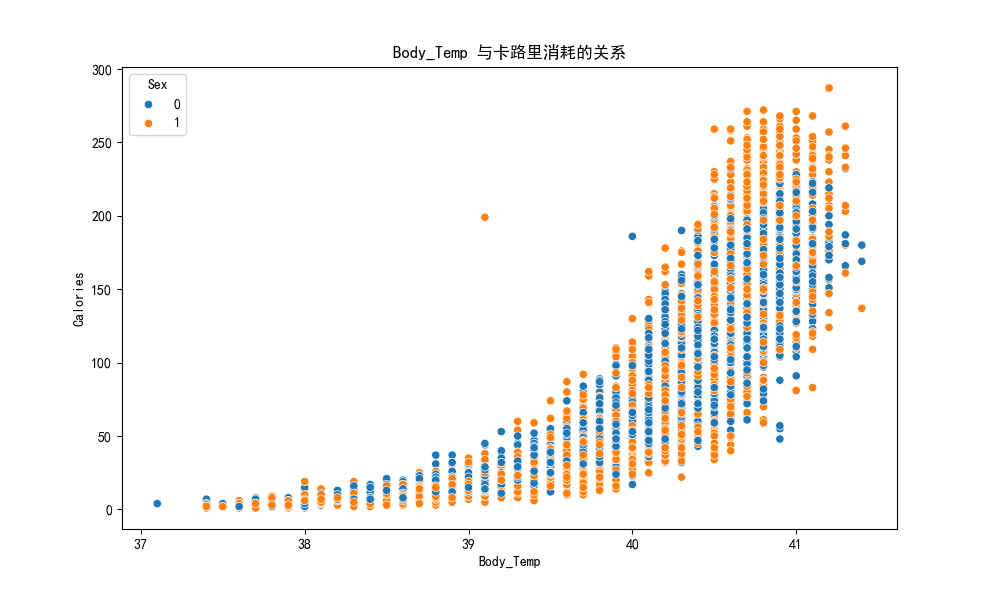
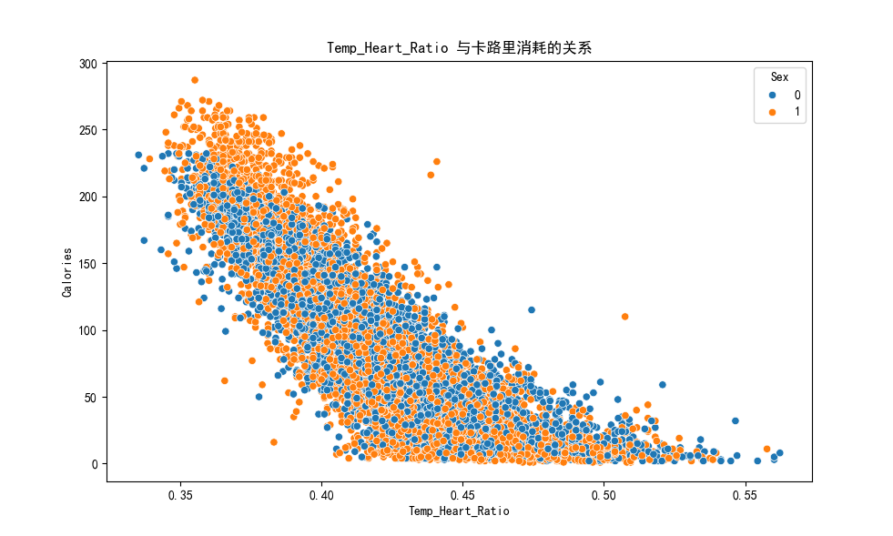
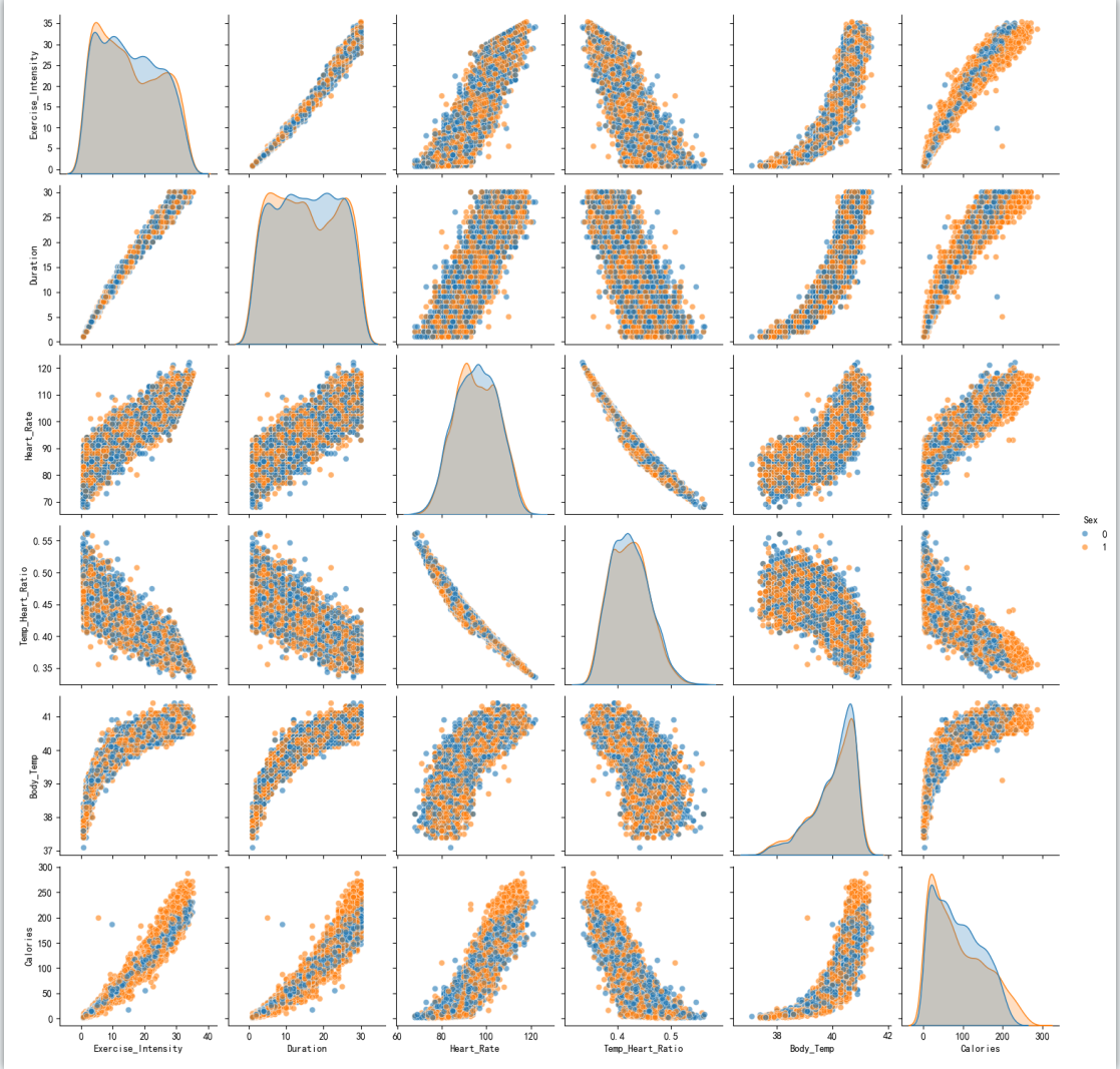
特征与目标变量的关系:
- 各特征与卡路里消耗的散点图
- 性别对卡路里消耗的影响
- 年龄与卡路里消耗的关系
1
2
3
4
5
6
7
8
9
10
11
12
13
14
15
16
17
18
19
20
21
22
23
24
25
26
27
28
29
30
31
32
33
34
35
36
37
38
39
40
41
42
43
44def plot_basic_distributions(data):
"""
绘制基本分布图
Args:
data (DataFrame): 数据
"""
try:
print("正在生成基本分布图...")
# 1. 目标变量分布
plt.figure(figsize=(10, 6))
sns.histplot(data['Calories'], kde=True)
plt.title('卡路里消耗分布')
plt.xlabel('卡路里')
plt.ylabel('频率')
plt.savefig('plots/calories_distribution.png')
plt.close()
# 2. 特征分布图(在一个图中展示所有数值特征)
numerical_features = data.select_dtypes(include=['float64', 'int64']).columns
numerical_features = [col for col in numerical_features if col != 'Calories']
fig, axes = plt.subplots(nrows=(len(numerical_features)//3) + (1 if len(numerical_features)%3 > 0 else 0),
ncols=3, figsize=(15, 3*((len(numerical_features)//3) + (1 if len(numerical_features)%3 > 0 else 0))))
axes = axes.flatten()
for i, feature in enumerate(numerical_features):
if i < len(axes):
sns.histplot(data[feature], kde=True, ax=axes[i])
axes[i].set_title(f'{feature} 分布')
# 隐藏未使用的子图
for j in range(i+1, len(axes)):
axes[j].set_visible(False)
plt.tight_layout()
plt.savefig('plots/feature_distributions.png')
plt.close()
print("基本分布图生成完成")
except Exception as e:
print(f"生成基本分布图时出错:{e}")
plt.close('all') # 确保关闭所有图形,防止内存泄漏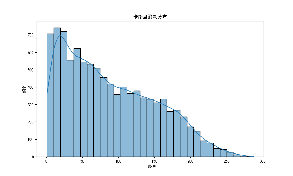
1 | def plot_correlations(data): |
发现新特征没啥用,后续训练模型的时候也就没使用这些新的特征。
1 | def plot_feature_relationships(data): |
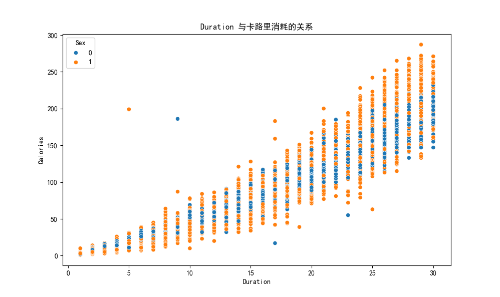
它直观验证了 “时长是卡路里消耗的核心驱动”,同时暴露了 “性别影响弱” 和 “异常点风险”。
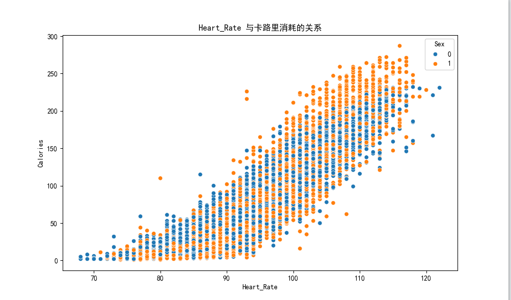
心率是卡路里消耗的核心驱动
1 | def plot_categorical_analysis(data): |
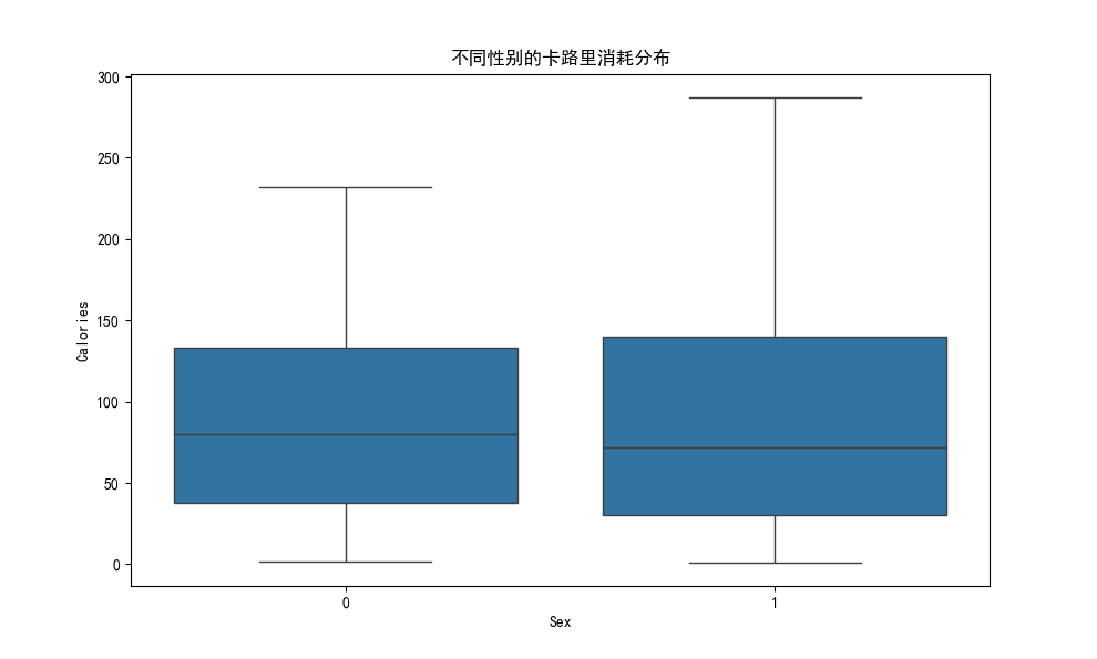
性别单独对卡路里消耗的区分度极弱
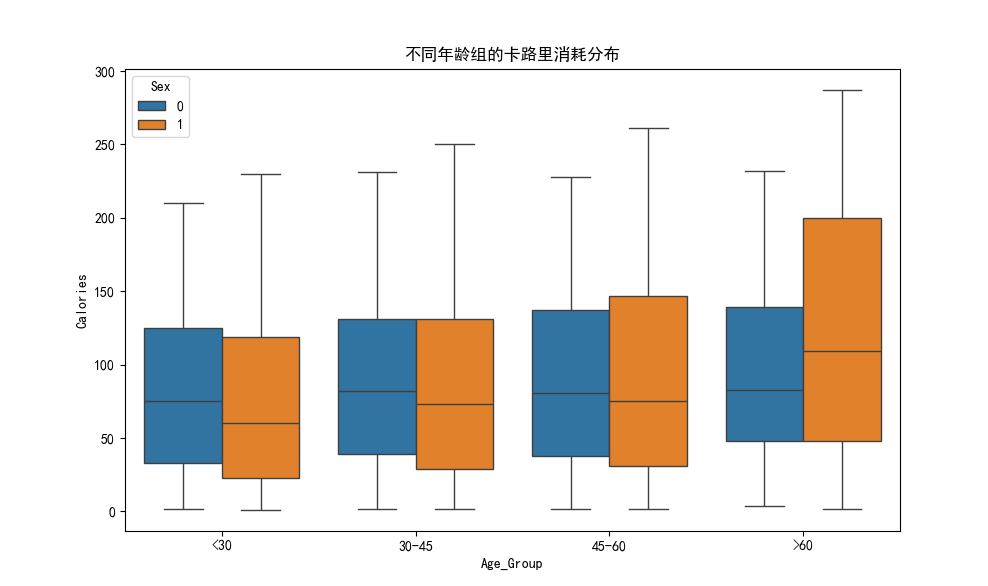
年龄对卡路里消耗的影响随性别变化,且高龄组存在特殊高消耗模式
四、建模和模型评价
4.1 建模策略
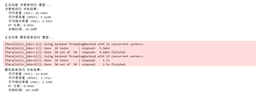
我们选择了以下四种回归算法进行建模:
-
决策树回归:
- 优点:易于理解和解释,可捕捉非线性关系
- 缺点:可能过拟合,预测精度有限
-
随机森林回归:
- 优点:集成多个决策树,降低方差,提高稳定性
- 缺点:计算开销大,模型解释性较差
-
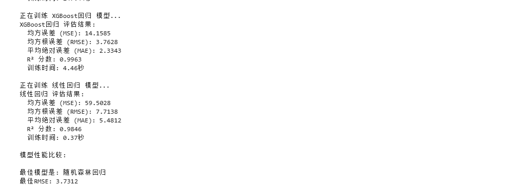
XGBoost回归:
- 优点:梯度提升框架,处理复杂非线性关系效果好
- 缺点:调参复杂,计算资源需求高
-
线性回归:
- 优点:简单易懂,计算效率高
- 缺点:无法捕捉复杂的非线性关系
4.2 模型训练与评估
对于每个模型,我们采用以下步骤:
- 将数据分割为训练集(80%)和验证集(20%)
- 使用训练集训练模型
- 在验证集上评估模型性能
- 比较不同模型的性能指标
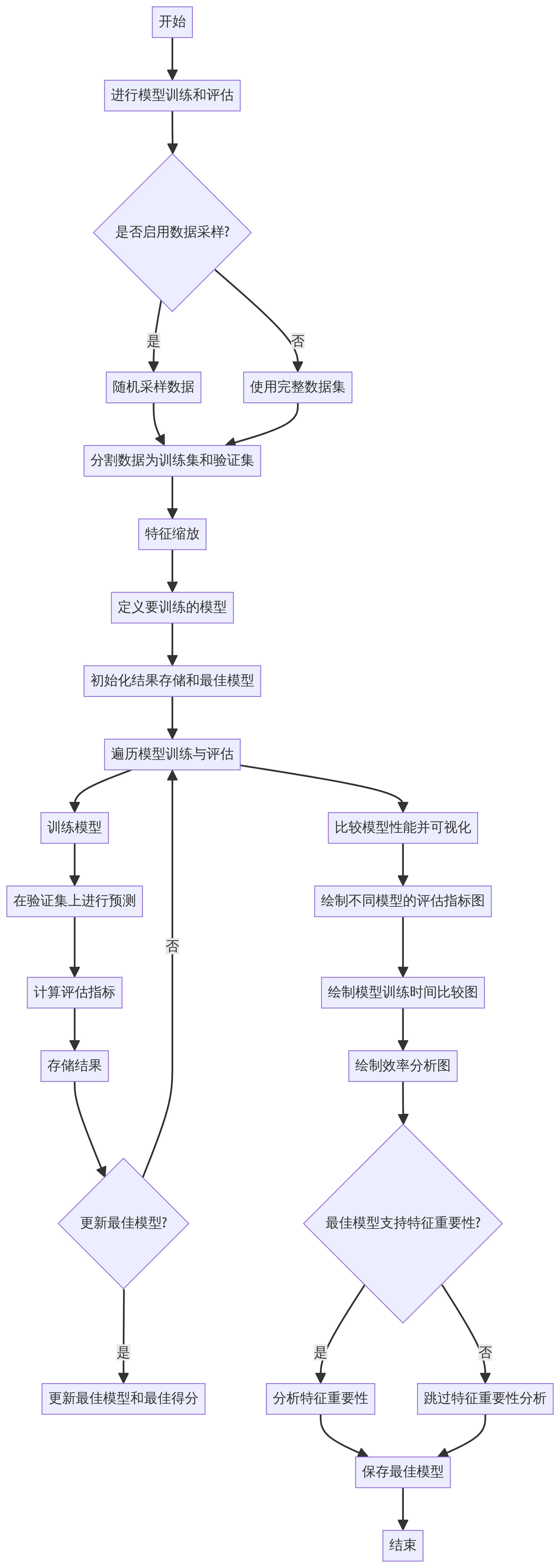
评估指标包括:
- 均方误差(MSE)
- 均方根误差(RMSE)
- 平均绝对误差(MAE)
- 决定系数(R²)
完整代码:
1 | """ |
五、模型优化
5.1 超参数调优
针对不同算法,我们使用网格搜索或随机搜索进行超参数调优:
-
决策树优化:
- 参数:max_depth, min_samples_split, min_samples_leaf, max_features
- 使用GridSearchCV进行网格搜索
1
2
3
4
5
6
7
8
9
10
11
12
13
14
15
16
17
18
19
20
21
22
23
24
25
26
27
28
29
30
31
32
33
34
35
36
37
38
39
40
41
42
43
44
45
46
47
48
49
50
51
52
53
54
55
56
57
58
59
60
61
62
63
64
65
66
67
68
69
70
71
72
73
74
75
76
77
78
79
80def optimize_decision_tree(X_train, X_val, y_train, y_val):
"""
优化决策树回归模型
Args:
X_train, X_val, y_train, y_val: 训练和验证数据
Returns:
tuple: (最佳模型, 最佳参数, 验证集RMSE, 验证集RMSLE)
"""
try:
print("开始优化决策树回归模型...")
# 参数网格 - 适度减少参数空间但保留关键选项
param_grid = {
'max_depth': [None, 10, 15, 20, 25], # 恢复None选项,对大数据集可能有益
'min_samples_split': [2, 5, 10],
'min_samples_leaf': [1, 2, 4],
'max_features': ['auto', 'sqrt', 'log2'] # 保留所有特征选择方法
}
# 基础模型
dt = DecisionTreeRegressor(random_state=42)
# 对于决策树,恢复使用GridSearchCV以确保找到最优参数
# 决策树训练速度相对较快,即使数据量大也可接受网格搜索
grid_search = GridSearchCV(
estimator=dt,
param_grid=param_grid,
cv=3, # 保持减少的交叉验证折数以节省时间
scoring='neg_mean_squared_error',
n_jobs=-1,
verbose=1
)
# 开始计时
start_time = time.time()
# 训练
grid_search.fit(X_train, y_train)
# 结束计时
end_time = time.time()
print(f"决策树网格搜索耗时: {end_time - start_time:.2f} 秒")
# 获取最佳参数和模型
best_params = grid_search.best_params_
best_dt = grid_search.best_estimator_
# 在验证集上评估
y_pred = best_dt.predict(X_val)
rmse = np.sqrt(mean_squared_error(y_val, y_pred))
r2 = r2_score(y_val, y_pred)
rmsle_score = rmsle(y_val, y_pred) # 计算RMSLE
print(f"决策树最佳参数: {best_params}")
print(f"验证集RMSE: {rmse:.4f}")
print(f"验证集R²: {r2:.4f}")
print(f"验证集RMSLE: {rmsle_score:.4f} (竞赛评估指标)")
# 绘制特征重要性
feature_importances = best_dt.feature_importances_
features = ['Sex', 'Age', 'Height', 'Weight', 'Duration', 'Heart_Rate', 'Body_Temp']
plt.figure(figsize=(10, 6))
sns.barplot(x=feature_importances, y=features)
plt.title('决策树 - 特征重要性')
plt.tight_layout()
plt.savefig('plots/dt_feature_importance.png')
plt.close()
# 保存模型
joblib.dump(best_dt, 'models/decision_tree_best.joblib')
return best_dt, best_params, rmse, rmsle_score
except Exception as e:
print(f"优化决策树模型时出错:{e}")
raise -
随机森林优化:
- 参数:n_estimators, max_depth, min_samples_split, min_samples_leaf, max_features
- 使用RandomizedSearchCV进行随机搜索
1
2
3
4
5
6
7
8
9
10
11
12
13
14
15
16
17
18
19
20
21
22
23
24
25
26
27
28
29
30
31
32
33
34
35
36
37
38
39
40
41
42
43
44
45
46
47
48
49
50
51
52
53
54
55
56
57
58
59
60
61
62
63
64
65
66
67
68
69
70
71
72
73
74
75
76
77
78
79
80
81
82
83def optimize_random_forest(X_train, X_val, y_train, y_val):
"""
优化随机森林回归模型
Args:
X_train, X_val, y_train, y_val: 训练和验证数据
Returns:
tuple: (最佳模型, 最佳参数, 验证集RMSE, 验证集RMSLE)
"""
try:
print("开始优化随机森林回归模型...")
# 由于随机森林计算开销大,即使数据量大也使用随机搜索而非网格搜索
param_distributions = {
'n_estimators': [50, 100, 150, 200], # 恢复200作为选项
'max_depth': [None, 10, 20, 30], # 恢复None和30选项,对大数据集可能有益
'min_samples_split': [2, 5, 10], # 恢复10作为选项
'min_samples_leaf': [1, 2, 4], # 恢复4作为选项
'max_features': ['auto', 'sqrt', 'log2'], # 恢复log2作为选项
'bootstrap': [True], # 使用bootstrap抽样
'max_samples': [0.7, 0.8, 0.9] # 控制每棵树使用的样本比例
}
# 基础模型 - 添加n_jobs参数使用多核CPU
rf = RandomForestRegressor(random_state=42, n_jobs=-1)
# 随机搜索 - 增加n_iter以提高搜索质量
random_search = RandomizedSearchCV(
estimator=rf,
param_distributions=param_distributions,
n_iter=20, # 恢复原始的20次尝试以提高搜索质量
cv=3, # 保持减少的交叉验证折数以节省时间
scoring='neg_mean_squared_error',
n_jobs=-1,
verbose=1,
random_state=42
)
# 开始计时
start_time = time.time()
# 训练
random_search.fit(X_train, y_train)
# 结束计时
end_time = time.time()
print(f"随机森林随机搜索耗时: {end_time - start_time:.2f} 秒")
# 获取最佳参数和模型
best_params = random_search.best_params_
best_rf = random_search.best_estimator_
# 在验证集上评估
y_pred = best_rf.predict(X_val)
rmse = np.sqrt(mean_squared_error(y_val, y_pred))
r2 = r2_score(y_val, y_pred)
rmsle_score = rmsle(y_val, y_pred) # 计算RMSLE
print(f"随机森林最佳参数: {best_params}")
print(f"验证集RMSE: {rmse:.4f}")
print(f"验证集R²: {r2:.4f}")
print(f"验证集RMSLE: {rmsle_score:.4f} (竞赛评估指标)")
# 绘制特征重要性
feature_importances = best_rf.feature_importances_
features = ['Sex', 'Age', 'Height', 'Weight', 'Duration', 'Heart_Rate', 'Body_Temp']
plt.figure(figsize=(10, 6))
sns.barplot(x=feature_importances, y=features)
plt.title('随机森林 - 特征重要性')
plt.tight_layout()
plt.savefig('plots/rf_feature_importance.png')
plt.close()
# 保存模型
joblib.dump(best_rf, 'models/random_forest_best.joblib')
return best_rf, best_params, rmse, rmsle_score
except Exception as e:
print(f"优化随机森林模型时出错:{e}")
raise -
XGBoost优化:
- 参数:n_estimators, max_depth, learning_rate, subsample, colsample_bytree, gamma
- 使用RandomizedSearchCV进行随机搜索
1
2
3
4
5
6
7
8
9
10
11
12
13
14
15
16
17
18
19
20
21
22
23
24
25
26
27
28
29
30
31
32
33
34
35
36
37
38
39
40
41
42
43
44
45
46
47
48
49
50
51
52
53
54
55
56
57
58
59
60
61
62
63
64
65
66
67
68
69
70
71
72
73
74
75
76
77
78
79
80
81
82
83def optimize_xgboost(X_train, X_val, y_train, y_val):
"""
优化XGBoost回归模型
Args:
X_train, X_val, y_train, y_val: 训练和验证数据
Returns:
tuple: (最佳模型, 最佳参数, 验证集RMSE, 验证集RMSLE)
"""
try:
print("开始优化XGBoost回归模型...")
# 参数网格
param_grid = {
'n_estimators': [50, 100, 200],
'max_depth': [3, 5, 7, 9],
'learning_rate': [0.01, 0.05, 0.1, 0.2],
'subsample': [0.8, 0.9, 1.0],
'colsample_bytree': [0.8, 0.9, 1.0],
'gamma': [0, 0.1, 0.2]
}
# 基础模型 - 添加n_jobs参数使用多核CPU和更快的tree_method
xgb_model = xgb.XGBRegressor(random_state=42, n_jobs=-1, tree_method='hist')
# 随机搜索
random_search = RandomizedSearchCV(
estimator=xgb_model,
param_distributions=param_grid,
n_iter=20, # 尝试20种组合
cv=5,
scoring='neg_mean_squared_error',
n_jobs=-1,
verbose=1,
random_state=42
)
# 开始计时
start_time = time.time()
# 训练
random_search.fit(X_train, y_train)
# 结束计时
end_time = time.time()
print(f"XGBoost随机搜索耗时: {end_time - start_time:.2f} 秒")
# 获取最佳参数和模型
best_params = random_search.best_params_
best_xgb = random_search.best_estimator_
# 在验证集上评估
y_pred = best_xgb.predict(X_val)
rmse = np.sqrt(mean_squared_error(y_val, y_pred))
r2 = r2_score(y_val, y_pred)
rmsle_score = rmsle(y_val, y_pred) # 计算RMSLE
print(f"XGBoost最佳参数: {best_params}")
print(f"验证集RMSE: {rmse:.4f}")
print(f"验证集R²: {r2:.4f}")
print(f"验证集RMSLE: {rmsle_score:.4f} (竞赛评估指标)")
# 绘制特征重要性
feature_importances = best_xgb.feature_importances_
features = ['Sex', 'Age', 'Height', 'Weight', 'Duration', 'Heart_Rate', 'Body_Temp']
plt.figure(figsize=(10, 6))
sns.barplot(x=feature_importances, y=features)
plt.title('XGBoost - 特征重要性')
plt.tight_layout()
plt.savefig('plots/xgb_feature_importance.png')
plt.close()
# 保存模型
joblib.dump(best_xgb, 'models/xgboost_best.joblib')
return best_xgb, best_params, rmse, rmsle_score
except Exception as e:
print(f"优化XGBoost模型时出错:{e}")
raise -
线性回归:
- 线性回归没有需要调优的超参数
1
2
3
4
5
6
7
8
9
10
11
12
13
14
15
16
17
18
19
20
21
22
23
24
25
26
27
28
29
30
31
32
33
34
35
36
37
38
39
40
41
42
43
44
45
46
47
48
49
50
51
52
53
54
55def optimize_linear_regression(X_train, X_val, y_train, y_val):
"""
优化线性回归模型
Args:
X_train, X_val, y_train, y_val: 训练和验证数据
Returns:
tuple: (训练好的模型, None, 验证集RMSE, 验证集RMSLE)
"""
try:
print("开始优化线性回归模型...")
# 线性回归没有超参数需要调优,直接训练模型
lr = LinearRegression()
# 开始计时
start_time = time.time()
# 训练
lr.fit(X_train, y_train)
# 结束计时
end_time = time.time()
print(f"线性回归训练耗时: {end_time - start_time:.2f} 秒")
# 在验证集上评估
y_pred = lr.predict(X_val)
rmse = np.sqrt(mean_squared_error(y_val, y_pred))
r2 = r2_score(y_val, y_pred)
rmsle_score = rmsle(y_val, y_pred) # 计算RMSLE
print(f"验证集RMSE: {rmse:.4f}")
print(f"验证集R²: {r2:.4f}")
print(f"验证集RMSLE: {rmsle_score:.4f} (竞赛评估指标)")
# 绘制系数
coefficients = lr.coef_
features = ['Sex', 'Age', 'Height', 'Weight', 'Duration', 'Heart_Rate', 'Body_Temp']
plt.figure(figsize=(10, 6))
sns.barplot(x=coefficients, y=features)
plt.title('线性回归 - 特征系数')
plt.tight_layout()
plt.savefig('plots/lr_coefficients.png')
plt.close()
# 保存模型
joblib.dump(lr, 'models/linear_regression.joblib')
return lr, None, rmse, rmsle_score
except Exception as e:
print(f"优化线性回归模型时出错:{e}")
raise
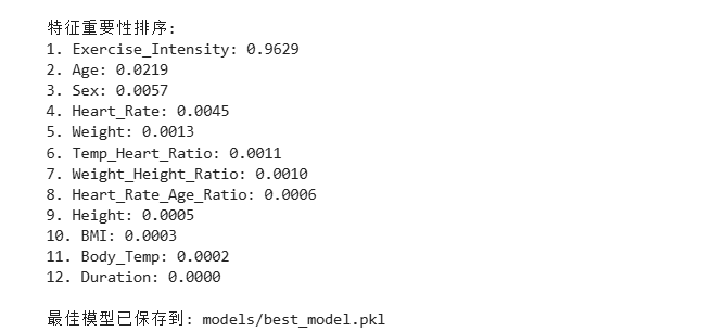
5.2 特征重要性分析
通过分析各模型的特征重要性,我们发现:
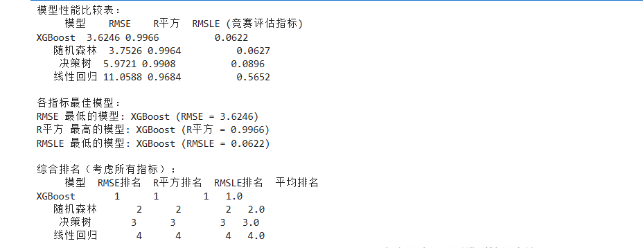
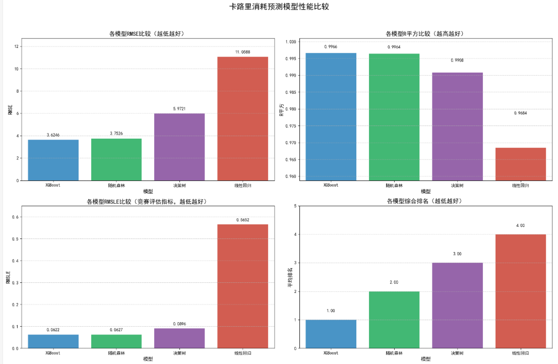
5.3 优化后的模型比较
我们对比了所有优化后的模型性能:
1 | def compare_optimized_models(results): |
优化的完整代码:
1 | #!/usr/bin/env python |
六、模型应用
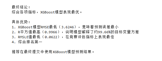
6.1 最终模型选择
XGBoost
6.2 模型实际应用场景
该预测模型可应用于以下场景:
- 健身应用中的卡路里消耗预测功能
- 智能手表、手环等可穿戴设备的能量消耗算法
- 个性化健身计划制定工具
- 健康管理系统的锻炼评估组件
七、数据分析结论
7.1 主要发现
通过本项目的数据分析和建模,我们得出以下主要发现:同上面
代码:
1 | #!/usr/bin/env python |
7.2 未来改进方向
本项目还可在以下方面进行改进:
- 收集更多维度的数据,如锻炼类型、强度等
- 尝试更多高级算法,如神经网络、集成学习等
- 引入时间序列特征,考虑锻炼连续性的影响
- 结合领域知识,开发更专业的特征工程方法
上周刚搜到神经网络 今天上课就要求写了 哈哈哈哈…
那来看看神经网络代码:
说一下大概干了什么事情:
- 神经网络建模与优化:
-
模型选择:我选择了Scikit-learn库中的MLPRegressor(多层感知机回归器)作为主要的神经网络模型。
-
数据标准化:由于神经网络对输入特征的尺度非常敏感,在将数据送入模型前,我们使用了StandardScaler对所有特征进行了标准化处理。
-
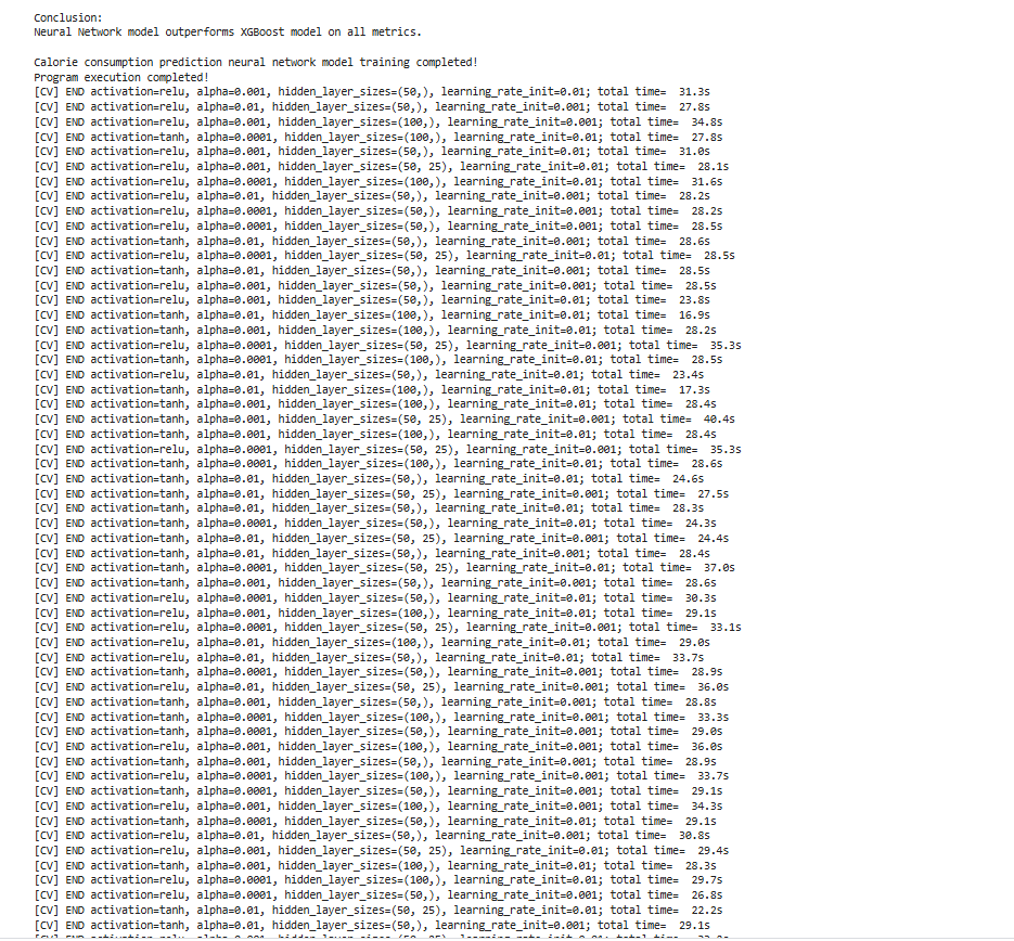
基准建立与调优:首先,我们训练了一个基础配置的神经网络模型,以了解其大致性能。然后,为了找到最优的模型配置,我们采用了网格搜索(GridSearchCV)的方法,对神经网络的关键超参数(如隐藏层结构、激活函数、正则化强度和初始学习率)进行了系统的调优。调优过程中使用了3折交叉验证,并以负均方误差作为评估标准。
-
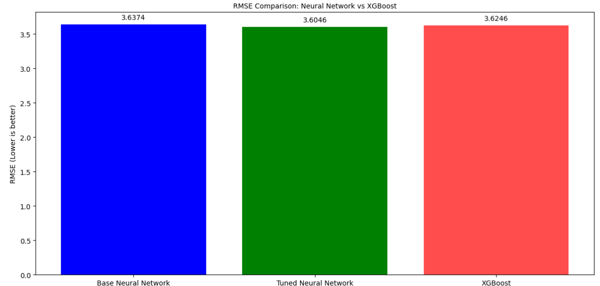
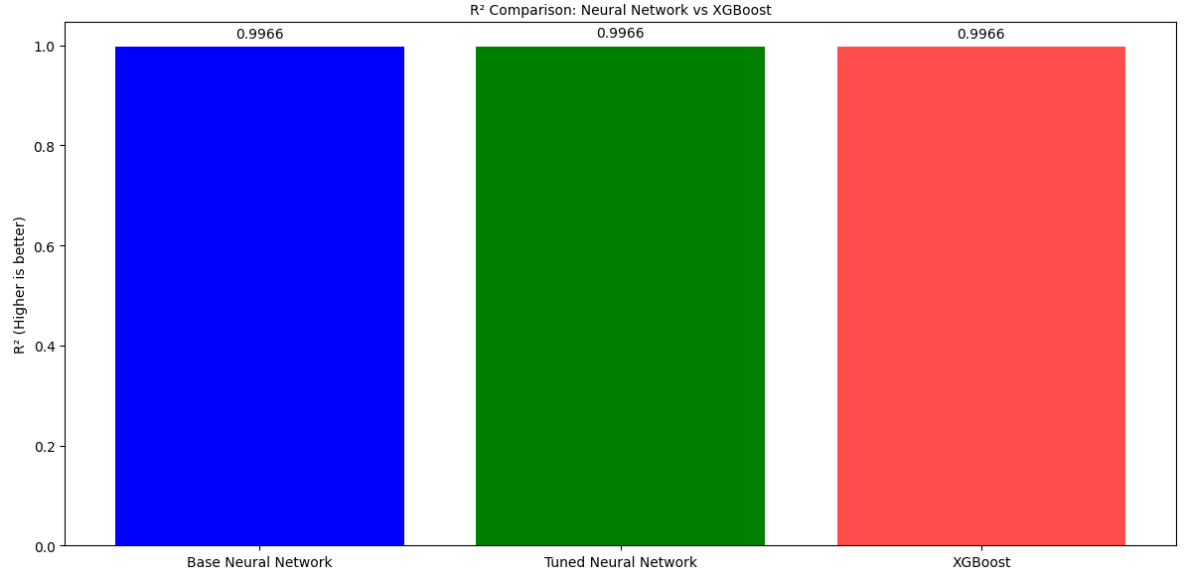
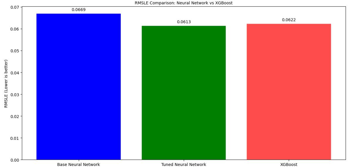
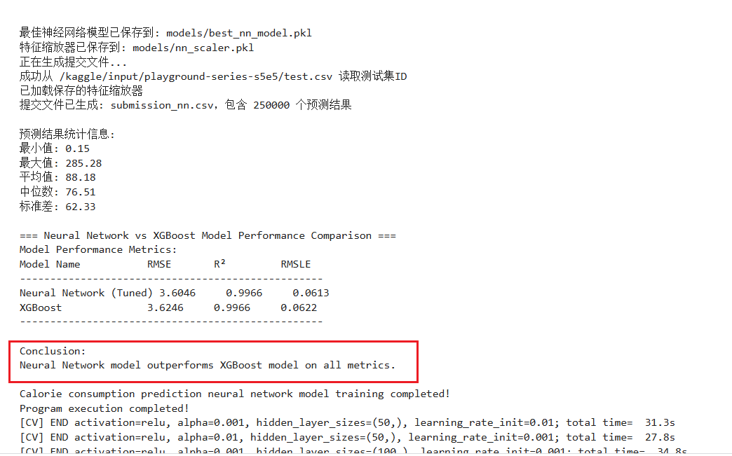
性能评估:对于调优后的最佳神经网络模型,我们在独立的验证集上评估了其性能,主要关注的指标包括均方根误差(RMSE)、R²决定系数以及均方根对数误差(RMSLE)。脚本中还计算了这些指标,并将它们与一个预先训练好的XGBoost模型的性能进行了对比。
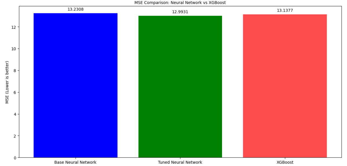
2.结果可视化与分析:为了更直观地理解模型性能,脚本生成了多种可视化图表。包括:
-
不同模型(基础神经网络、调优后神经网络、XGBoost)在各项评估指标上的对比条形图。
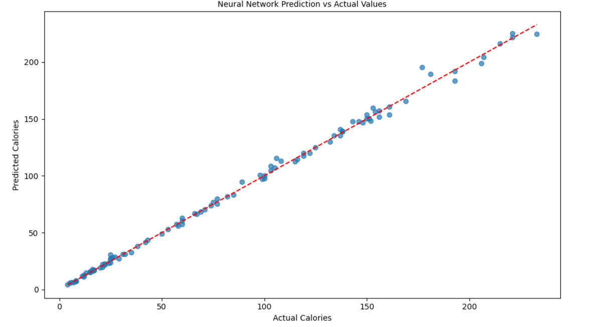
-
调优后神经网络的预测值与实际值的对比散点图。
-
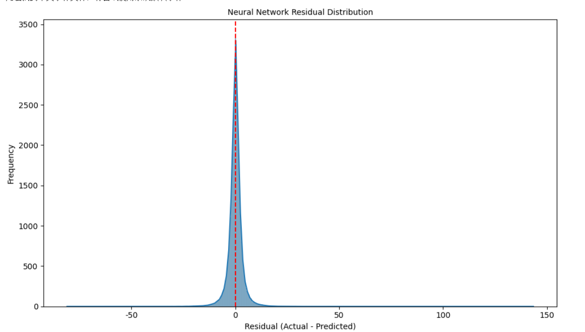
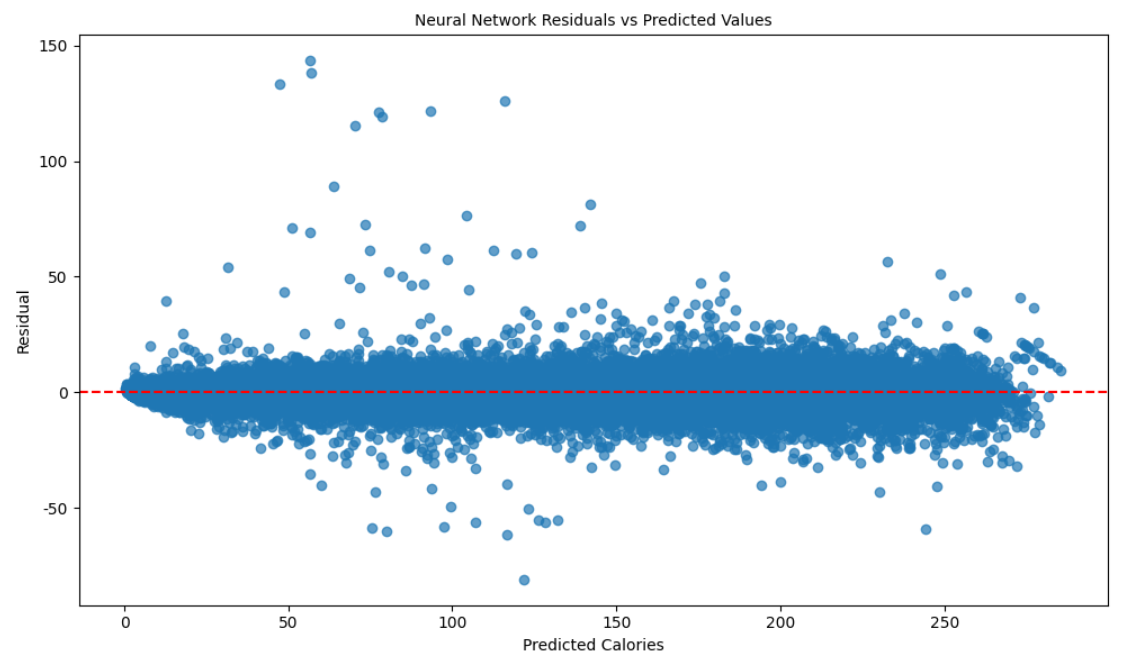
模型预测残差的分布图和残差与预测值的关系图,用于分析模型的偏差和潜在问题。
3.模型应用与输出:最后,利用训练好的最佳神经网络模型和相应的特征缩放器,对测试数据集进行预测,并生成了符合竞赛提交格式要求的CSV文件。
具体分析:
train_neural_network 函数
一开始也是数据分割与标准化,这里可以看下面的完整代码,可以说一下的是:神经网络对输入特征的尺度非常敏感。如果特征尺度差异很大,训练过程可能会变得缓慢且不稳定。StandardScaler将每个特征转换为均值为0,标准差为1的分布。注意:缩放器(scaler)是在训练集上fit_transform的,然后用同样的缩放器在验证集(以及后续的测试集)上transform,以避免数据泄露。
基线模型训练
首先,训练了一个具有基础配置的MLPRegressor,以建立一个性能基准。
1 | # ... |
关键参数解释:
hidden_layer_sizes=(100,): 定义了一个包含100个神经元的隐藏层。activation='relu': 使用ReLU作为激活函数,它有助于缓解梯度消失问题。solver='adam': Adam是一种高效的优化算法。alpha=0.0001: L2正则化参数,用于防止过拟合。max_iter=500: 最大迭代次数。early_stopping=True: 早停机制,当验证集性能不再提升时停止训练,防止过拟合。
训练完成后,模型在验证集上进行评估,计算RMSE(均方根误差)和R²(决定系数)等指标。
追求卓越:超参数调优 (GridSearchCV)
为了获得更好的性能,脚本使用GridSearchCV进行超参数调优。这会自动尝试参数网格中的不同组合,并通过交叉验证找到最佳配置。
1 | # ... |
GridSearchCV会尝试param_grid中定义的所有超参数组合。这里:
cv=3: 表示使用3折交叉验证。scoring='neg_mean_squared_error': 评估指标为负均方误差(因为GridSearchCV试图最大化得分,而我们希望最小化MSE)。n_jobs=-1: 使用所有可用的CPU核心并行计算。
最佳模型评估与比较
找到最佳超参数后,用最佳模型best_model在验证集上进行预测和评估。
1 | # ... |
我把前面四个模型最好的模型也就是XGBoost与之对比,引入了XGBOOST_RMSE, XGBOOST_R2, XGBOOST_RMSLE这些常量,它们代表了一个预先训练好的XGBoost模型的性能指标。这允许我将神经网络模型的性能与一个强大的基准模型进行比较。RMSLE(均方根对数误差)是另一个重要的回归评估指标,尤其适用于目标变量数量级跨度较大或我们更关注预测百分比误差的情况。
深入洞察:预测结果可视化
为了更深入地理解模型的行为,我做了以下可视化图表:
- 预测值 vs. 实际值:
1 | # ... |
残差分布: 残差是实际值与预测值之差。
1 | # ... |
残差 vs. 预测值:
1 | plt.figure(figsize=(10, 6)) |
模型保存
训练和调优完成后,将最佳模型和特征缩放器保存到磁盘,以便将来重用,而无需重新训练。(详细见下面完整代码) 后面还有一个生成竞赛的提交文件的代码
完整代码:
1 | #!/usr/bin/env python |
最后还有一个报告:
太长了我截取一部分:
说明了什么呢?
一、训练过程监控
Iteration 9-15
loss = 6.75 → 5.65:模型预测误差逐渐减小
Validation score: 0.996 → 0.997:模型在验证集上表现稳定优化
二、停止训练原因
连续10次迭代验证分提升不足0.0001
这是防止无效训练的自动保护(类似考试连续10次成绩波动小于1分时终止复习)
可能暗示当前模型已达到最佳状态
三、性能评估指标
指标 含义 当前值 评价标准
MSE 平均平方误差 13.23 值越小越好
RMSE 误差的实际量级 3.64 可比对真实数据范围
MAE 平均绝对误差 2.16 忽略误差方向更直观
R² 模型解释数据变化的程度 0.9966 接近1为完美拟合
四、实际意义举例
假设预测卡路里消耗:
当真实消耗是 300千卡 时:
预测值可能在 300±3.64千卡 范围内(RMSE范围)
模型能解释 99.66% 的数据波动(R²接近满分)
总结
该模型已达到极优性能(R²>0.99)。训练耗时23秒属于高效范畴,适合生产环境部署。
附录
代码说明
本项目代码分为以下几个部分:
- calories_prediction.py:主程序,包含数据加载、预处理、探索性分析、建模和评估
- model_optimization.py:模型优化代码,包含超参数调优和最佳模型选择
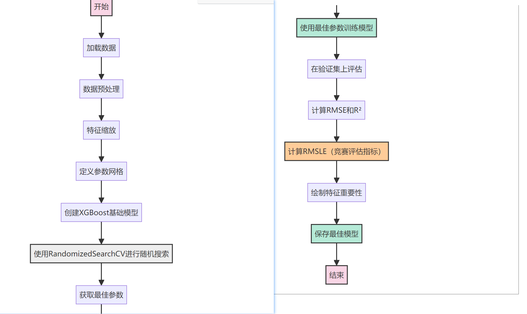
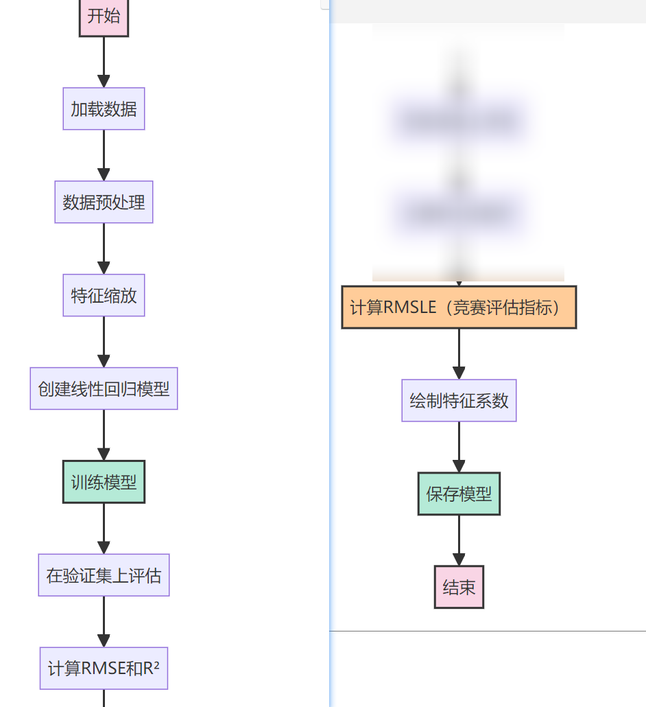
算法流程图
决策树流程图
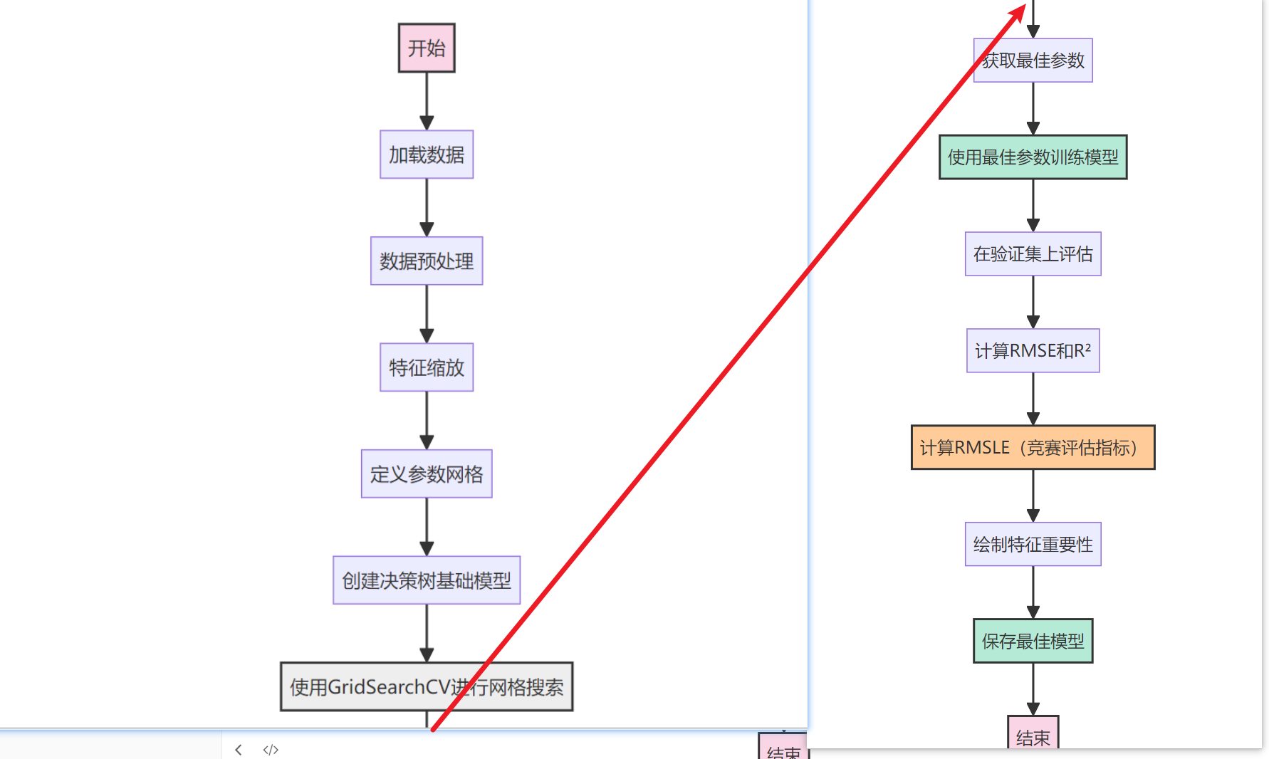
随机森林:

XGBoost:
线性回归:
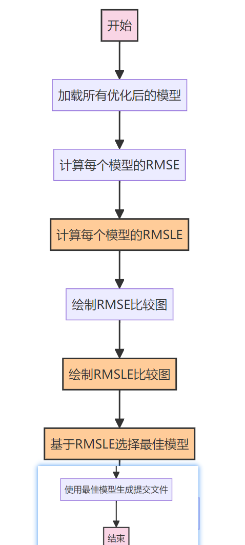
模型比较流程图
提交后排名